 |
Introduction |
|
Changing climates are expected to severely alter the phenology, growth, mortality/regeneration and eventually composition of tree species in Switzerland, Europe and worldwide. Severe climate extremes (abrupt shifts) and slowly altering climate means (gradual shifts) have started to affect these demographic responses (Gehrig-Fasel et al. 2007; Jolly et al. 2005; Lenoir et al. 2008; Menzel & Fabian 1999; van Mantgem et al. 2009). While over short periods (next 10-20 years) the effect of land use change and changes in phenology may still dominate the climate signal in its importance at the landscape scale, ongoing climate change with an increased frequency of extremes and more dramatically shifted means is expected to outweigh land use change thereafter, and severe alterations in growth, regeneration and mortality of individual tree species may be expected and can partly be observed already today (Kurz et al. 2008; Rigling et al. 2006). And several species have already undergone recent range shifts (Parmesan & Yohe 2003; Walther et al. 2002).
Forecasting the effects of climate change on species responses bears the difficulty that no single method will give easy answers to the many questions resulting from the uncertainty about ongoing climate change. It seems thus reasonable to evaluate possible effects of climate change from an array of methods. Often used are species distribution models (SDMs) to evaluate the geographical re-displacement of suitable habitat areas for species (Iverson et al. 2008; Thuiller et al. 2005; Zimmermann et al. 2006). Other methods assess the impact of climate variability on phenology (Menzel & Fabian 1999), growth (Jolly et al. 2005), regeneration (Ibanez et al. 2007), or mortality (Bigler et al. 2006; van Mantgem & Stephenson 2007; van Mantgem et al. 2009; Villalba & Veblen 1998). Common garden transplants are an alternative, yet very resource intense approach (Rehfeldt 1991).
Species Distribution and Climate Change
The method of SDM (Guisan & Thuiller 2005; Guisan & Zimmermann 2000) is suited to analyze possible effects of climate change on species, since it assesses the macro-scale climate suitability of a species under altered climate (Thuiller et al. 2008). Specifically, for sessile organisms as plants, the suitability of a site for sustainable growth and maintenance of viable populations is highly important and has the potential to assist managers in decision making regarding the selection of species for forestry, conservation biology and landscape planning. The method has matured and a general agreement has been reached as to what degree the many statistical methods are capable of fitting species' distributions along environmental gradients (Elith et al. 2006; Guisan et al. 2007). Many additional effects have been evaluated, such as the importance of sample size (McPherson et al. 2004; Pearce & Ferrier 2000; Stockwell & Peterson 2002; Zimmermann et al. 2007), sampling design (Edwards et al. 2006), or to what degree specific sets of additional predictors, such as remote sensing variables (Pottier et al. 2014; Zimmermann et al. 2007), biotic variables (Kissling et al. 2012; Leathwick & Austin 2001), or the inclusion of climatic extremes (Zimmermann et al. 2009) help explain species distributions. Additional emphasize has been given to the modeling of the potential distribution of rare species, since small sample sizes clearly pose difficulties (Edwards et al. 2005; Guisan et al. 2006).
Tree Growth and Climate change
Various site and environmental factors determine tree growth. As summarized earlier (Kozlowski & Pallardy 1996), the requirements for tree growth are carbon dioxide, water, and minerals for raw materials, light as energy resource, oxygen, and favorable temperature for growth processes. The capacity for photosynthetic processes (i.e. foliar biomass) and the competition for resources are constraining tree growth. Tree growth processes can be ranked by order of importance in foliage growth, root growth, bud growth, storage tissue growth, stem growth, growth of defensive compounds, and reproductive growth (Waring 1987). The growth potential is further influenced by tree species interactions, tree genetics (local adaptation, seed origins), tree age, and stand density and structure (Kramer 1988). In temperate forests the potential vegetation period (determined by the seasonal global radiation budget) is limited by temperature (Kozlowski & Pallardy 1996).
Past provenance trials in Switzerland have shown that tree growth (both in tree height and volume) decreases in general with increasing altitude for the same provenances and tree species (Burger 1941; Dobbertin & Giuggiola 2006). While temperature is expected to be the most important explaining variable, other factors such as soil type, soil mineralization rate or wind and snow may also contribute to the decline in growth with altitude. However, similar decreases in tree growth were found in all the provenance trials and gradient studies Burger conducted. By using a mean temperature lapse rate of 0.6°C per 100 m change in altitude Burger's findings can be translated into height and stem increment decreases of 5-10% for Norway spruce (Picea abies) and 5-20% for Scots pine (Pinus sylvestris) per 1°C of temperature decrease (Dobbertin & Giuggiola 2006).
Long-term phenological observations show for deciduous trees that leaf duration has increased by up to two weeks in Europe over the past thirty years due to increasing temperatures (Menzel & Fabian 1999). Given sufficient water and nutrient suppl, rising temperatures are therefore believed to increase forest growth. However, several studies found poor relations between leaf duration and stem growth (Jolly et al. 2005; Kaufmann et al. 2004; Leuzinger et al. 2005; White & Nemani 2003). Hasenauer and colleagues (Hasenauer et al. 1999) found for the time period 1961-1990 a parallel increase in mean annual temperature, computed growing season and actual stem growth and modelled net primary productivity on the Austrian national forest inventory grid indicating a causal relation between temperature increase and growth increase. In a European wide study using 5-year growth data from 363 ICP Forests level II plots, Solberg et al. (2009) found not only a strong effect of nitrogen deposition on tree growth, but also of deviation of the temperature during the vegetation season from the long-term mean. Andreassen et al. (2006) found in Norway that spruce plots with a 30-years mean June temperature value below 12-13°C mostly reacted with increased growth when the summer weather was drier or warmer than normal, and vice versa. In summary, the poor relation between leaf duration and stem growth likely can be explained by the fact that early season warming does not necessarily relate directly to increased productivity. Rather, seasonal productivity changes are driven by the interplay between rising temperatures and changes in water availability, which is further outlined below.
The provenance trials described above had all been conducted in regions that were not limited by precipitation. In some dry inner-alpine valleys (such as the Rhone valley) tree height actually increases with increasing altitude related to increasing precipitation and decreasing temperature with altitude (Dobbertin & Giuggiola 2006). It is well established that tree stem growth is affected by the water availability during the growing season and previous years (Schweingruber 1996; Spiecker 1990; Spiecker et al. 1996). The severe drought during the temperature record-setting summer 2003 in Europe (Schär et al. 2004) also affected stem growth at long-term monitoring sites in Germany and Switzerland (Ciais et al. 2005; Jolly et al. 2005; Meining et al. 2004). Meining et al. (2004) report reduced stem diameter growth rates by an average of 50% in 2003 for all 10 Norway spruce Level II sites in Baden-Württemberg. In Bavaria growth in 2003 for all seven Level II spruce sites was reduced in comparison to 2002 (Meining et al. 2004). For European beech (Fagus sylvatica), growth reduction was also found at low altitude sites (510 to 780 m), but above 800 m beech showed no growth reduction. In Switzerland, tree growth of 2003 in percent of growth in 2002 decreased irrespective of species with decreasing altitude. At low altitude (<1200 m) tree growth was reduced on average by one third compared to the wet year 2002 (Dobbertin & Giuggiola 2006), while the trees on plots above 1200 m a.s.l. exhibited increased stem growth (mean of 15%, Dobbertin & Giuggiola 2006) most likely due to increased temperatures (Jolly et al. 2005).
How to interpret projected range shifts
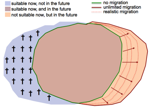
Species distribution models (SDM) fit the observed current distribution of a species to a range of climate and other predictors. When projecting this model to change climate scenario maps, rapid - basically immediate - range shifts are projected (Figure 1). Several points need to be considered when interpreting this type of model output:
Figure 1. Schematic representation of shifts in suitable habitats from species distribution models. Three zones can usually be distinguished, depending on whether the habitat is projected to be suitable now and/or in the future.
(1) A projected range shift by - say - 2080 does not mean that the species is expected to ultimately go extinct in the whole range that no longer is simulated to be suitable (blue part in figure 1). Rather, the model says that "under current climate conditions, the species has not been observed with sufficient evidence under such conditions the species might experience in the future at these locations". This only answers that there is no evidence the species should be there in the long run. But it does not answer, how fast the species will disappear. If the future climate conditions impose direct physiological stress, then the species might disappear fast (as can e.g. be observed with Scots pine in the lowest altitudes of the Valais, where in the recent two decades the species has disappeared do to increased drought extremes. However, in many cases a species will still find physiologically suitable conditions. It is rather the competition with better performing species that will result in range loss over time. Such competition based range shifts take 100s if not 1000s of years, and can also be mitigated by forest management.
(2) Each model has zones of errors. There is no "error-free" model. In SDMs we always expect errors to be visible at the edge of the distribution. It does not mean that just outside (or just inside) of the predicted edge we expect the species to disappear/appear. Rather, it is a probabilistic model, and we optimize the cut level in order to have better visualization capacity (and because probabilities are also difficult to interpret). Yet, it's clear that we expect most deviations from the true reality at range edges.
(3) SDMs as produced here are fitted from all forest inventory points across the European Alps. This has the advantage that all possible habitat conditions under which the species can be observed in the Alps are used to fit the niche model. This guarantees that the model more broadly represents the full niche of the species. However, it has the disadvantage that it does not give sufficient attention to Swiss data points. The plots in Switzerland may stand for local adaptation of Swiss provenances that are not equally well captured when fitting a model with all data points of the Alps. We may specifically see differences to Swiss inventory points for species that have their center of distribution outside of Switzerland (the Swiss provenances might represent local adaptations to conditions at the edge of the distribution; see e.g. Ostrya carpinifolia), or for species that have a very broad environmental niche (see e.g. Pinus sylvestris). We consider the advantage of fitting a more complete niche of the species as very high due to the need to predict to conditions we cannot currently observe in Switzerland. This requires fitting models for a larger range of current climate conditions.
(4) Due to fact that we fit models over the whole European Alps has one significant disadvantage, though. The lack of Alps-wide soil, geology, or land-use data prevents us from calibrating these important environmental variables into the models. To overcome this, we can only fit models for Swiss data alone, where these environmental predictors are available. Most of the presented species are fitted directly at the Alps-scale. Only models of few species that cannot be successfully predicted from the Alps-wide data basis are calibrated from Swiss data alone, in order to assess their likely future response under climate change. These models are clearly assigned as fitted from Swiss data in Appendix S1. This allows to easily recognize the different model calibration reference. When fitting Swiss data points alone, we have added three predictor variables: (i) a categorical geology variable (calcareous vs. non-calcareous bedrock), (ii) soil depth, and (iii) distance to water (standing or running).
(5) In appendix S1 we present a range change statistic for each species at the Swiss and in many cases at the European scale. The European scale is meant to represent the whole European continent. These statistics are only available for some of the modeled species, and were calculated from models originating from the EU FP7 MOTIVE project. The models were calibrated using the ICP Forest Level I plots, a network of ca. 6500 plots allocated in a ca. 16km regular lattice over forest areas of Europe. If a species has only a Swiss range statistic, then no European models were available for this species.
(6) Not all national forest inventories that we used in this project distinguish the tree species always to the species level. Some countries failed to distinguish specifically the different species of oaks (Quercus spp.), maples (Acer spp.) and ash (Fraxinus spp.). Instead of fitting Alps-wide models for the individual species from some selected regions only (which would have biased clearly the model calibration), we decided to present only the genus level models. For oaks, the models lump generally the species Q. robur, Q. petraea, and Q. pubescens (but not Q. ilex, nor Q. cerris). For maples, the models generally combine the specie A. pseudoplatanus, A. platanoides, and A. campestre. For ashes, the models combine the species F. excelsior and F. ornus.
References
|
© 1998-2024 WSL - - Last Update: Fri Oct 30 2020