
18.09.2025 | Michael Haugeneder | SLF News
Contact 
Not only did the Arctic ice melt away from under our feet at record-breaking speed, but the expedition also flew by far too quickly. Since the beginning of September, we have been back at the institute and going about our "normal" business. All too soon we are back in the daily grind and it is all the more important to recapitulate promptly and to put the new findings into a scientific context and write them down. So it seems like a good time to write the third and final part of this expedition blog.
This text was automatically translated.
As global warming progresses and the ice extent and concentration decreases from year to year, the Arctic and the Arctic ecosystem are undergoing major changes. Where there used to be permanent, thick ice, today there are sometimes only pitiful remnants. It is clear that the changes in the polar regions have global climatic consequences. In order to assess the consequences of these changes, we need to understand the processes involved. The CONTRASTS expedition aimed to do just that. CONTRASTS because the aim is to show the differences between various ice regimes - the ice of today, the ice of the future and the ice of the past.
The typical ice of the present forms in the central Arctic, is part of the transpolar drift and is a mix of one- and two-year ice. The ice of the future will unfortunately only be seasonal ice; forming in winter and completely melting away in summer. The ice of the past is characterized by multi-year ice; ice that forms and survives for several years, for example in the Beaufort Gyre system.
No sooner said than done. We approached the three chosen ice floes from the different zones four times each with the Polarstern, whereby the first ice floe from the edge zone unfortunately did not survive the third round. It broke into pieces and drifted into Russian territory. This meant that the measuring buoys installed on the floe were actually lost, but thanks to drifting back into Norwegian waters, we were able to fish most of them out of the water again. The autonomous measuring buoys were just one thing. The other, and already known from previous blog posts, were our measurements on the floes. One of our two main focuses was to physically characterize the "mysterious material" on the sea ice. What looks like snow from a distance actually has little to do with the snow we know from the Alps. Scientifically, it is called the "surface scattering layer" (SSL). This layer is also formed from the snow that falls in winter, but is mainly characterized by the melting and freezing processes of salt and fresh water and the changes in the freeboard with the associated "flooding and draining". Thanks to the physical similarities to snow, however, we can still use our familiar snow measuring devices and methods. The main aim of CONTRASTS is to statistically record the difference between the ice regimes and the heterogeneity of the individual floes in order to be able to parameterize the processes in climate models more precisely. Our task is therefore to measure the heterogeneity of the surface properties of the snow or the SSL, and anyone who is familiar with statistics will quickly realize that the more diligently and the more we measure, the better the statistics will be. And we took this to heart and tried to make the most of every minute on the ice. Of course, there were days when we wished we were at home and cursed the umpteenth measurement on a Transect. To be honest, holding a device on the snow surface a thousand times, pressing a button and then waiting five seconds until you can move to the next measurement position can be quite monotonous. It was certainly an advantage that the three of us already knew each other very well and were able to motivate each other on days when we had a lull.
The second focus was on the measurements with the screen and the thermal imaging camera to measure the turbulent heat flows near the ground. The permanently high humidity and ice formation on the screen were definitely limiting factors, which meant that it was no longer possible to measure the air temperature undisturbed. Nevertheless, we set up the measuring device on each floe, but only stretched out the screen itself when the expedition meteorologist's forecasts were promising. The expedition leader even kept the entire crew waiting for us and delayed our onward journey so that we could take advantage of a short, forecast fog-free weather window. With a somewhat guilty conscience, there were three of us and a bear guard on the ice and we were very relieved when the fog finally lifted and we were able to take measurements for another two hours.
We returned home satisfied with a large number of measurements. The individual measurements are nothing exciting in themselves. However, as the first evaluations of these countless measurements show, there are clear differences between the ice regimes and in the seasonal progression. Although the expedition and the field work were really exciting and varied, the real thriller is only just beginning. Analyzing the data, linking your own data with ocean, ice or atmospheric data in order to understand the processes - this is where the second part of the work begins. And this is where the researcher's heart definitely beats faster.

Image 1 of 14
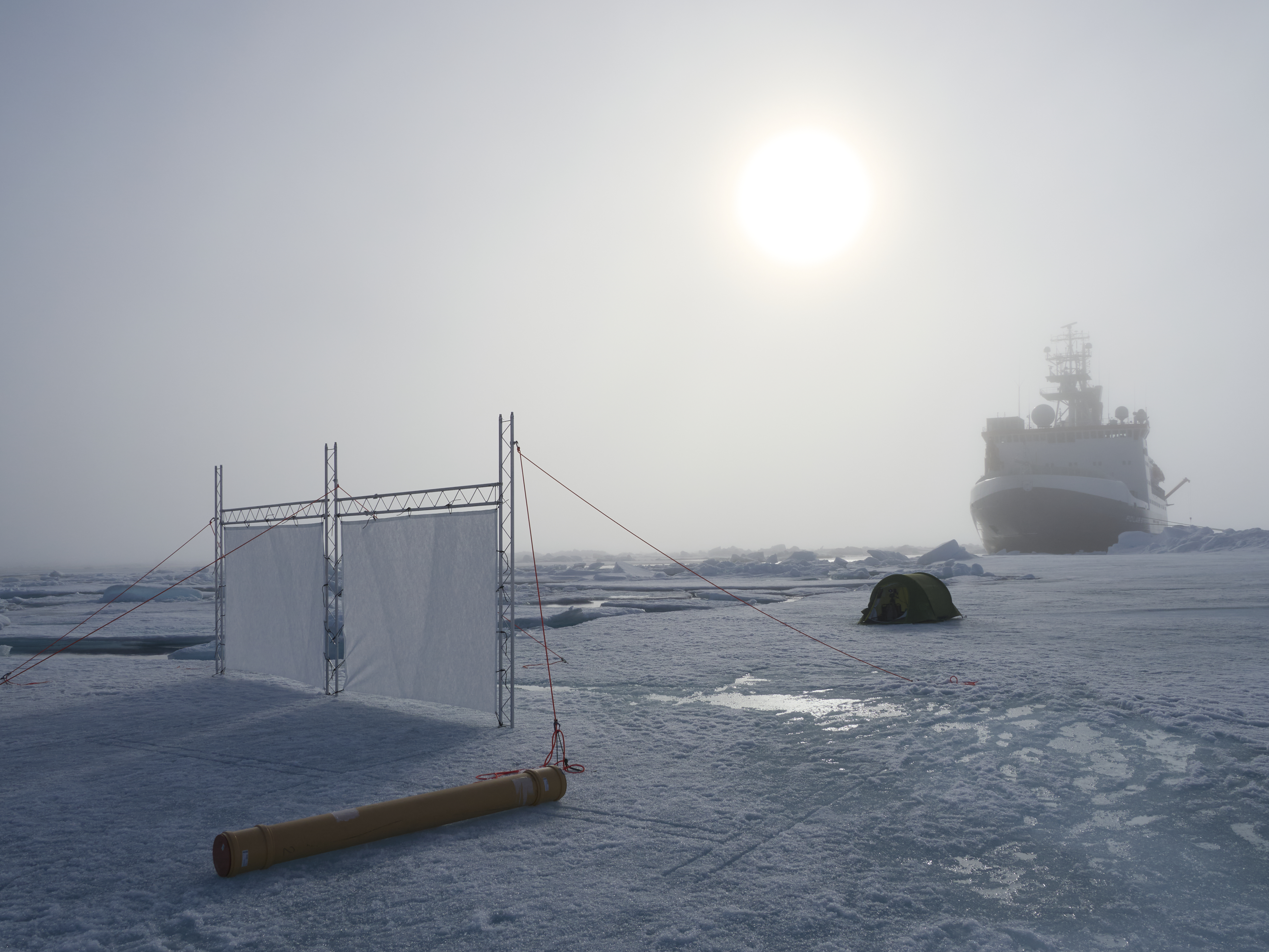
Setting up the screen for measuring turbulent heat flows. The frequently prevailing foggy conditions meant that the screen was often icy, preventing the measurement from working. As a result, we often only hung up the screen once the fog had lifted. (Photo: Matthias Jaggi / SLF)

Image 2 of 14
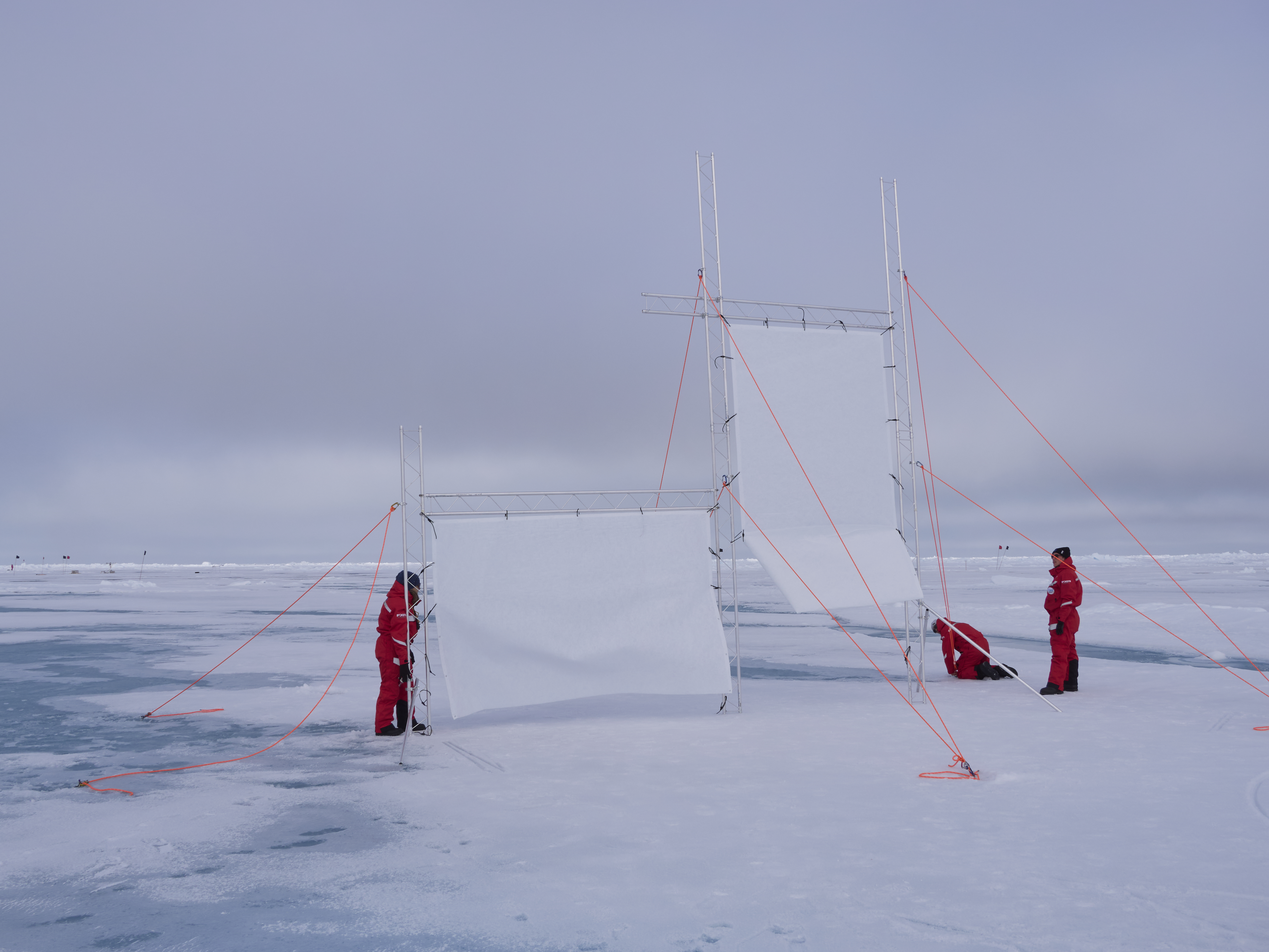
Hanging up the screen as soon as the weather conditions regarding wind speed and risk of icing have calmed down. (Photo: Matthias Jaggi / SLF)

Image 3 of 14
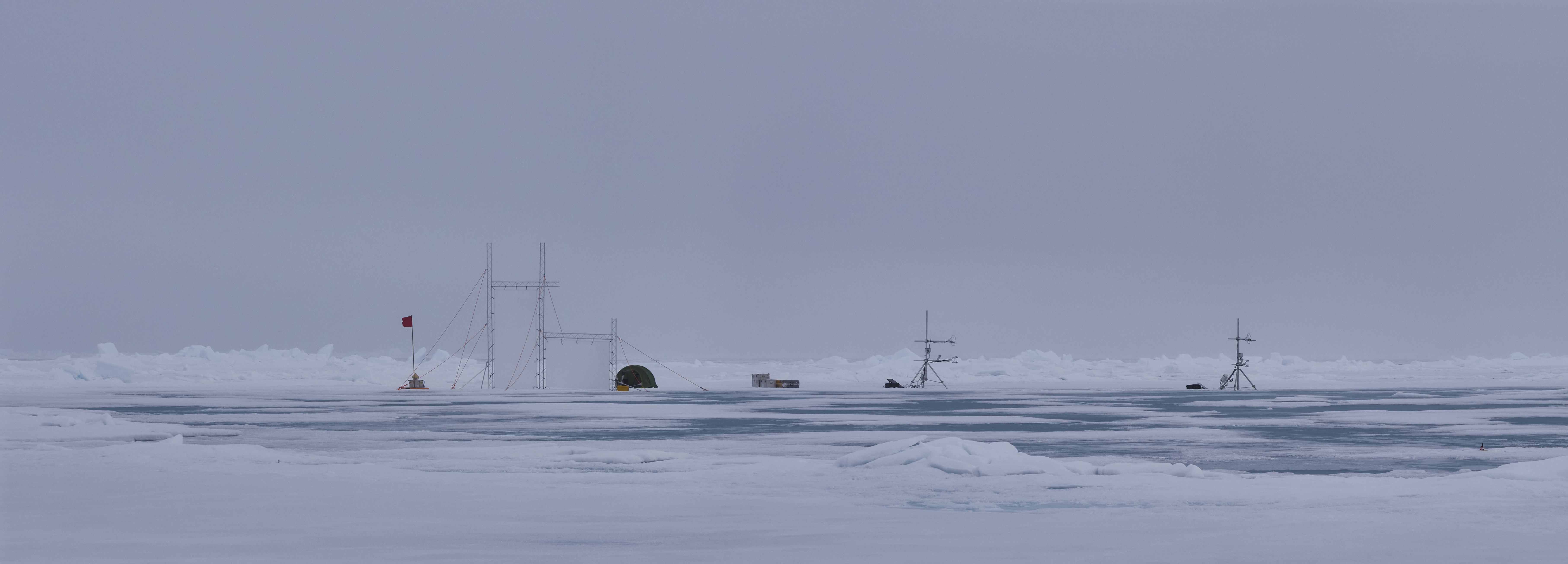
Complete measurement setup for turbulent heat flows at the transition from melt pools to snow. In addition to the screen and the thermal imaging camera protected in the tent, there were also two wind stations. (Photo: Matthias Jaggi / SLF)

Image 4 of 14
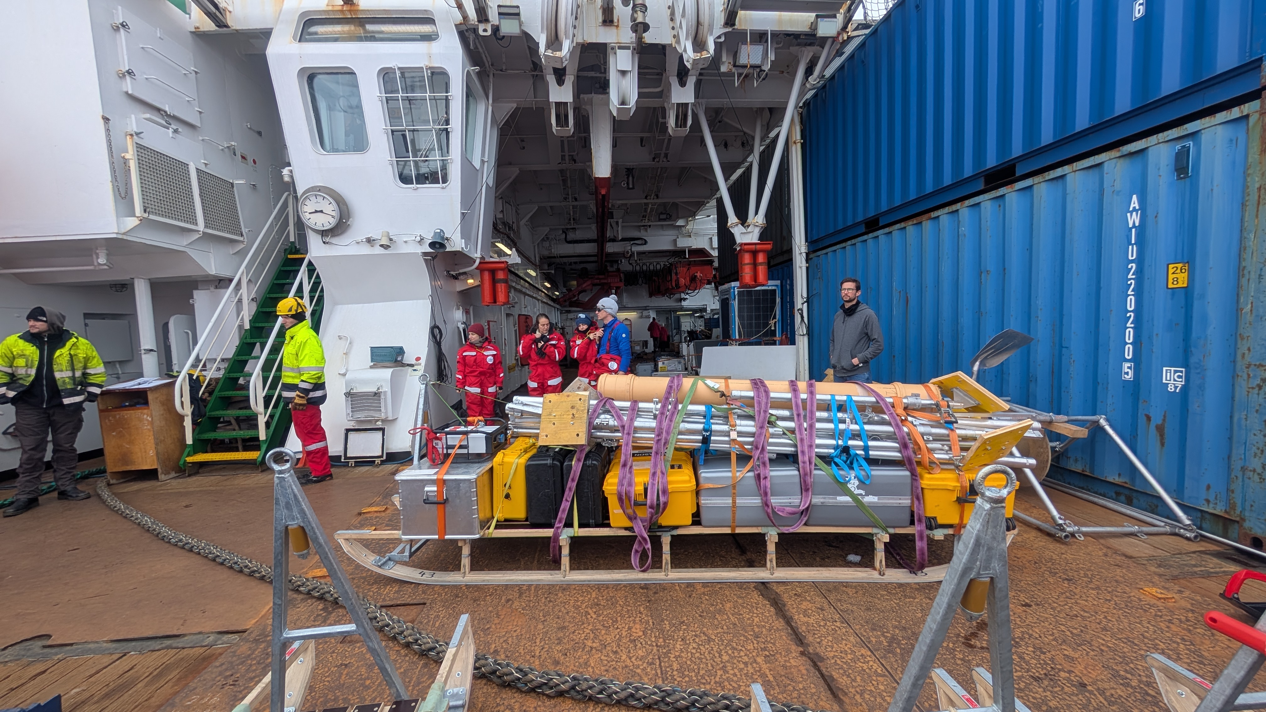
Nansen sled with all the equipment needed for turbulent heat flux measurements. Before arriving at each ice floe, we packed the sled so that it could be lifted onto the ice using a ship's crane. This enabled us to get started immediately upon arrival and lose as little measurement time as possible. (Photo: Matthias Jaggi / SLF)

Image 5 of 14
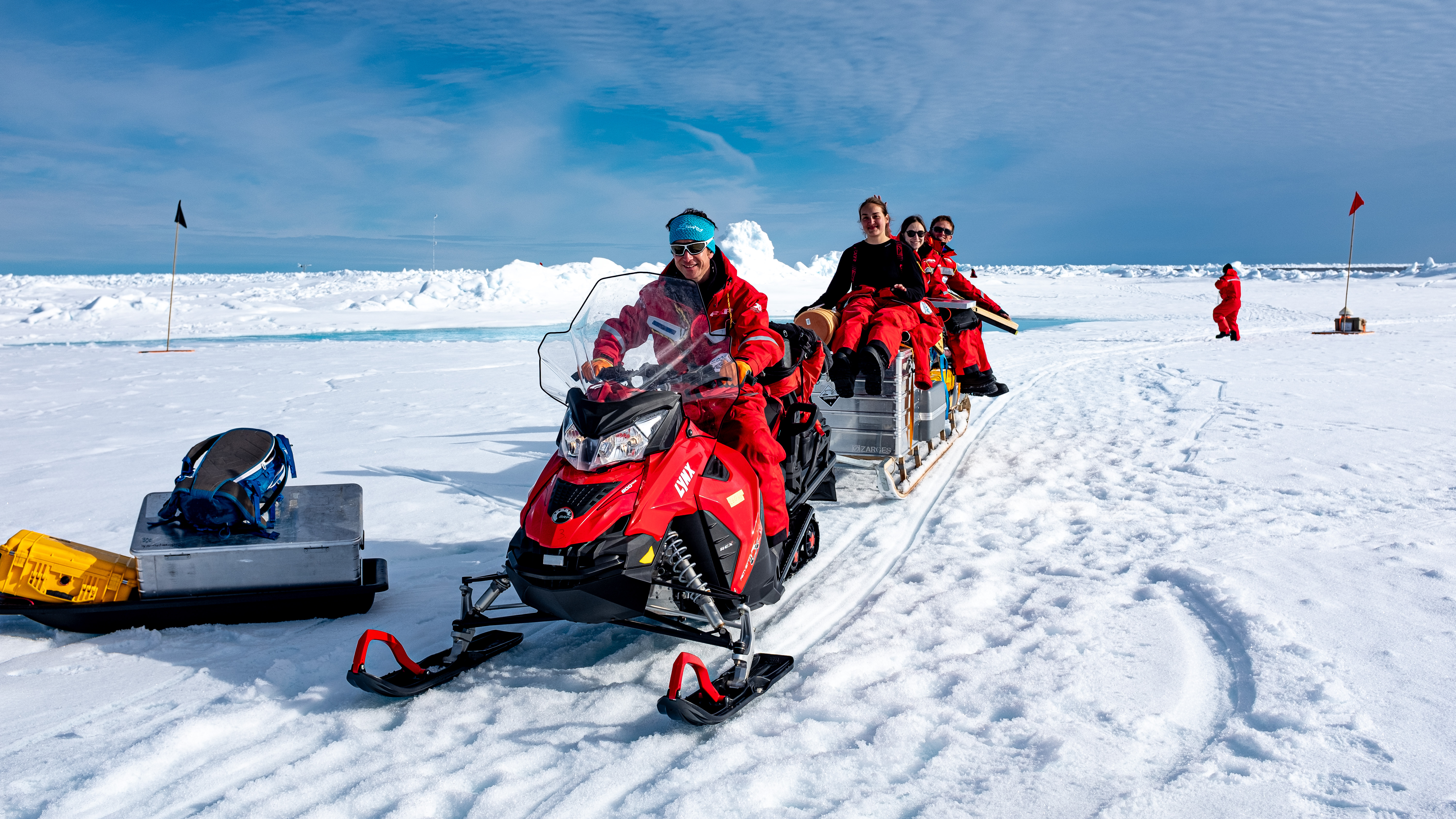
In the ‘good’ cases, we were able to drive the Nansen sled to the desired measuring location with the Skidoo. However, if the distances were short or the ice strength was not beyond doubt, we simply pushed the sled by hand. (Photo: Ruzica Dadic / SLF)

Image 6 of 14
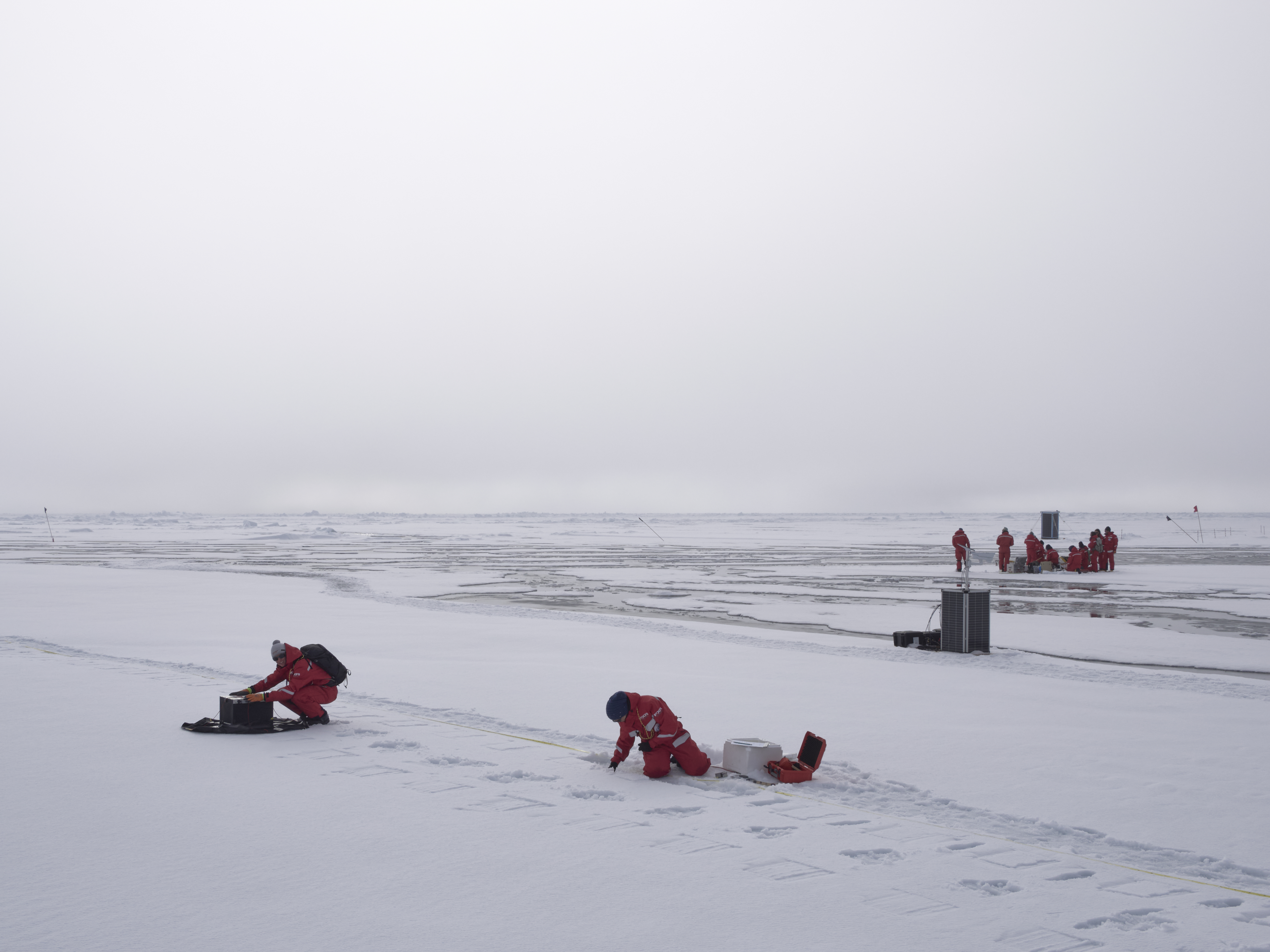
Successive measurements on a defined transect. Shown here are reflectance measurements with the SnowImager and parallel snow profiles under relatively homogeneous surface conditions. (Photo: Matthias Jaggi / SLF)

Image 7 of 14
SnowImager measurements on a defined transect with greater heterogeneity. Here, the transition from snow-covered conditions to a frozen melt pool. The albedo of these two different surfaces will differ by orders of magnitude, which will be reflected in the SnowImager measurements. (Photo: Matthias Jaggi / SLF)

Image 8 of 14
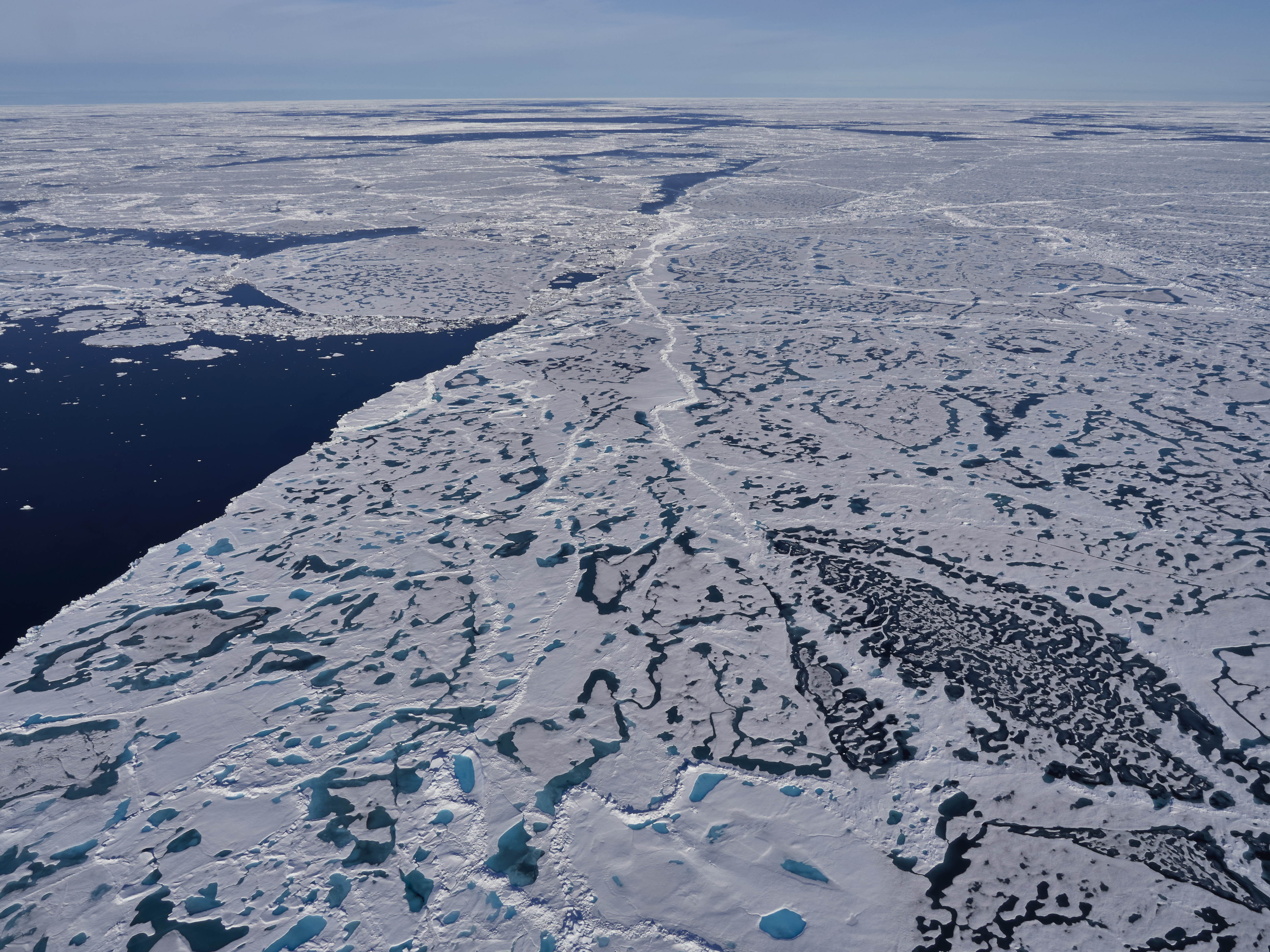
Heterogeneity of ice conditions during the summer melt phase. From a bird's eye view, it quickly becomes clear that surface properties cannot be specified with a single value. (Photo: Matthias Jaggi / SLF)

Image 9 of 14
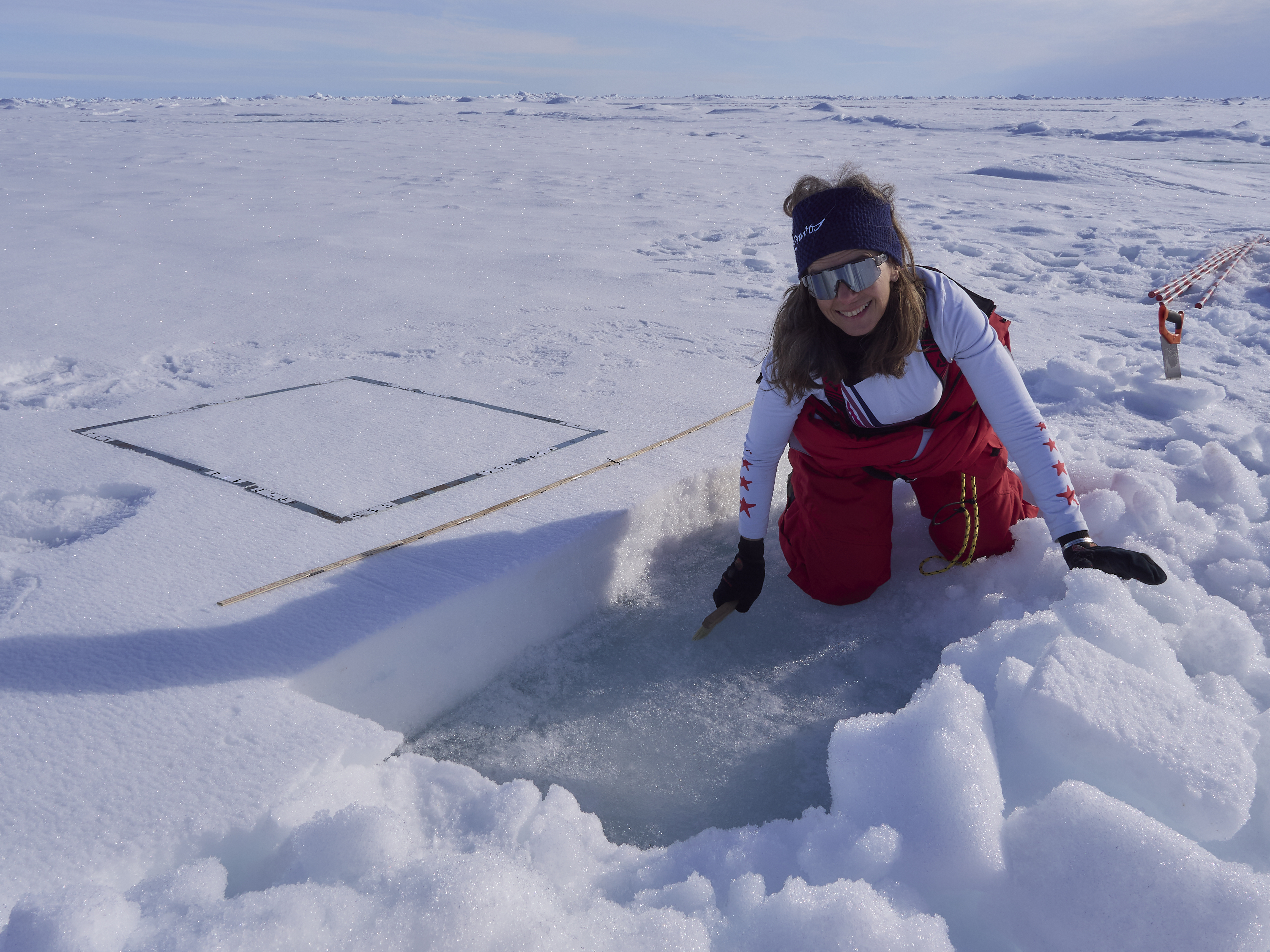
Quasi-traditional snow profile on sea ice. Typical ‘snow depths’ were in the range of a few centimetres. We rarely got to dig properly, but were all the more delighted when there was more. (Photo: Matthias Jaggi / SLF)

Image 10 of 14
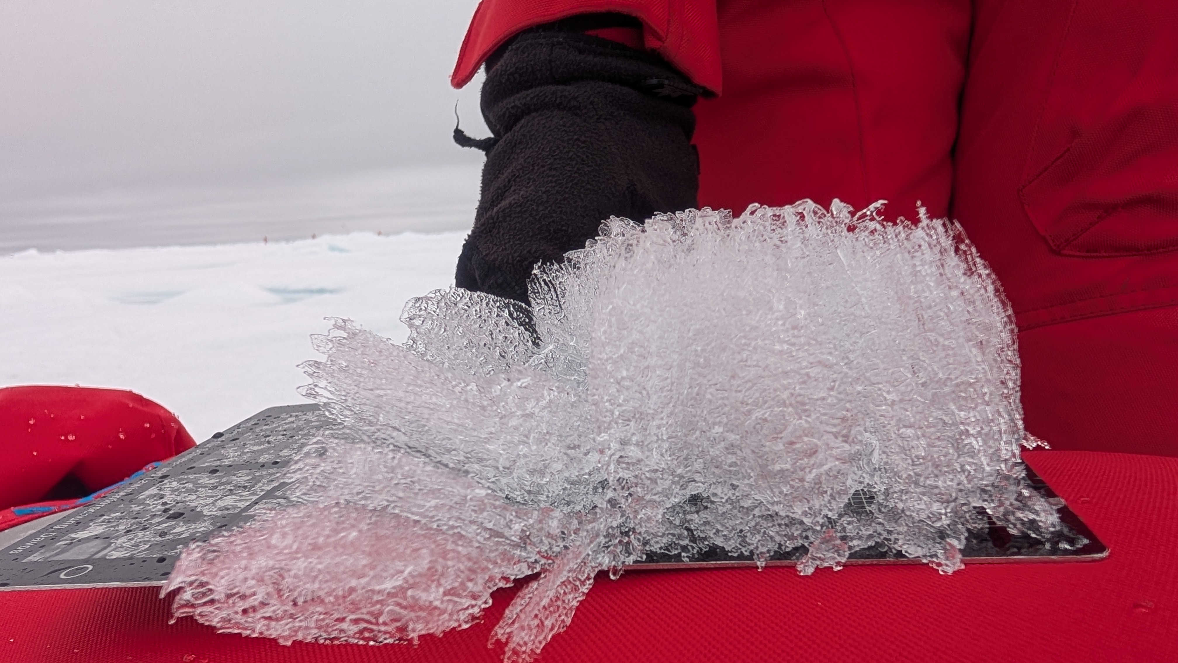
Surface scattering layer. Centimetre-sized ice structures with fine channels. In order to perform computer tomography on such structures, we had to patiently cut out cylindrical samples with a diameter of 9 centimetres without destroying them. (Photo: Matthias Jaggi / SLF)

Image 11 of 14
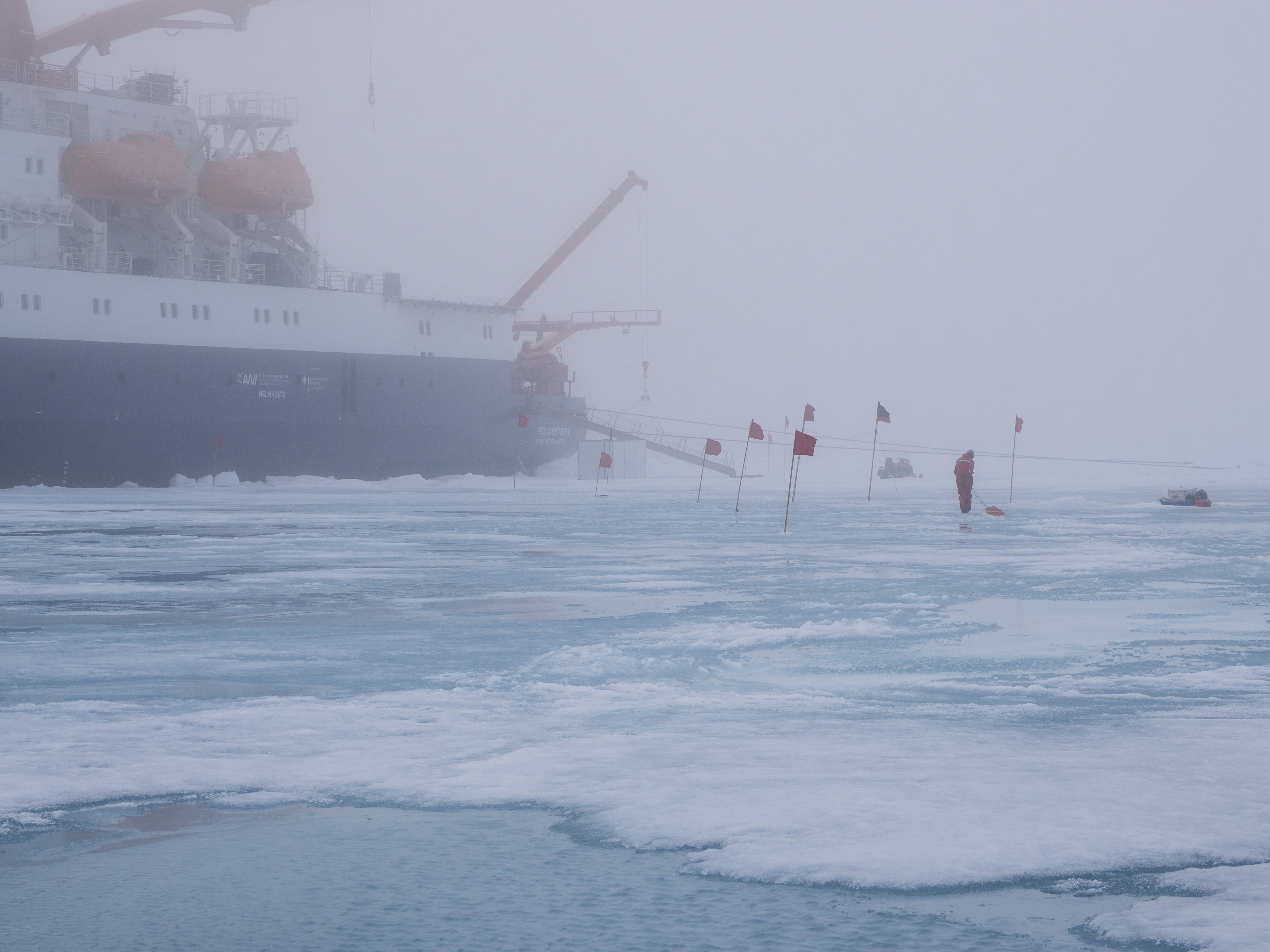
Our ‘old lady’. The Polarstern is our home during the expedition. Normally, the Polarstern would have been anchored in the ice with ropes. However, as the ice here was already very thin, the anchors would not have held, which is why the ship used its thrusters to constantly push itself slightly against the edge of the ice. (Photo: Matthias Jaggi / SLF)

Image 12 of 14
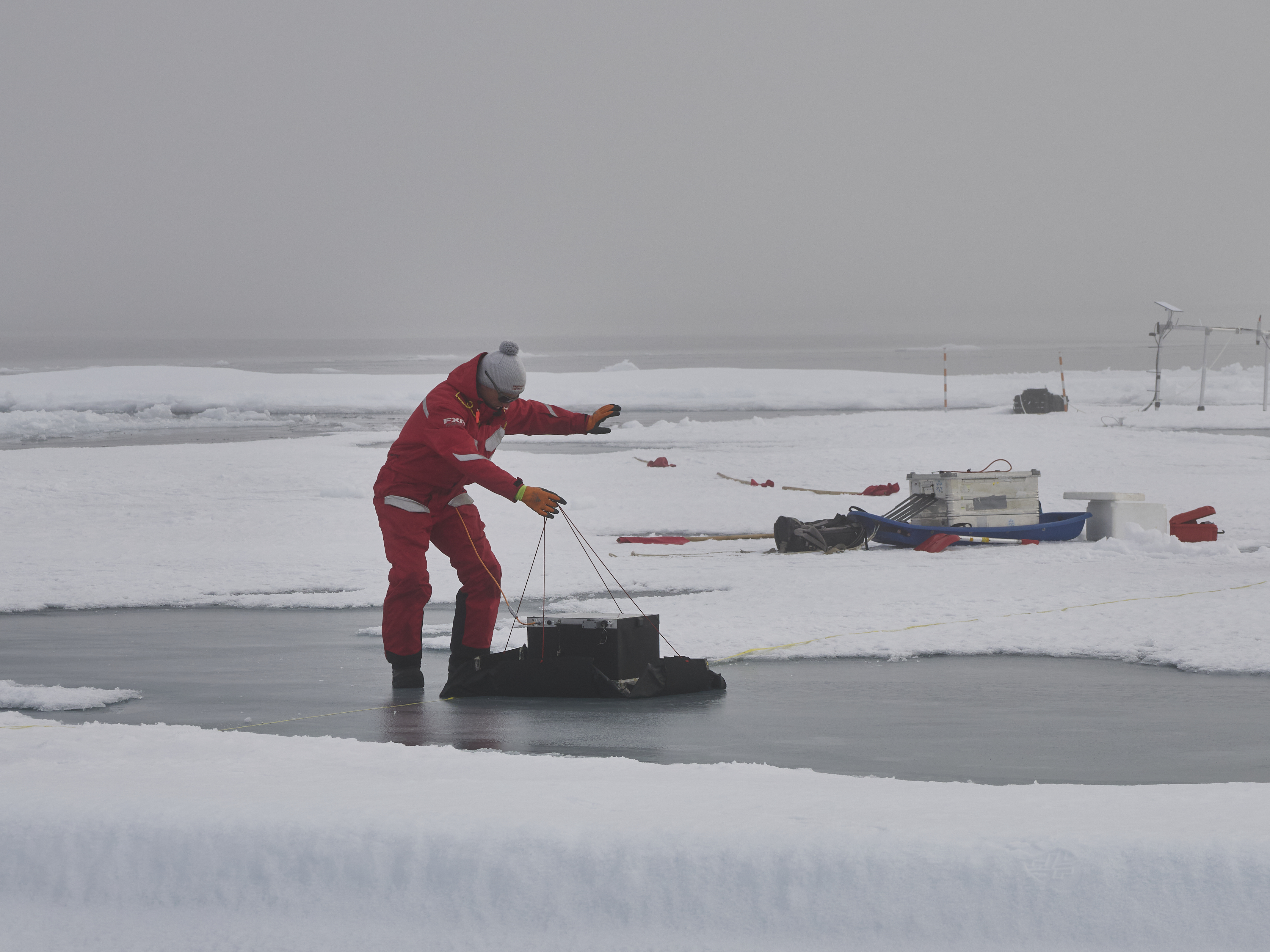
Summer melting conditions on the ice floe. Here, you often have to find your way between the ship and the measuring station to avoid getting wet feet. (Photo: Matthias Jaggi / SLF)

Image 13 of 14
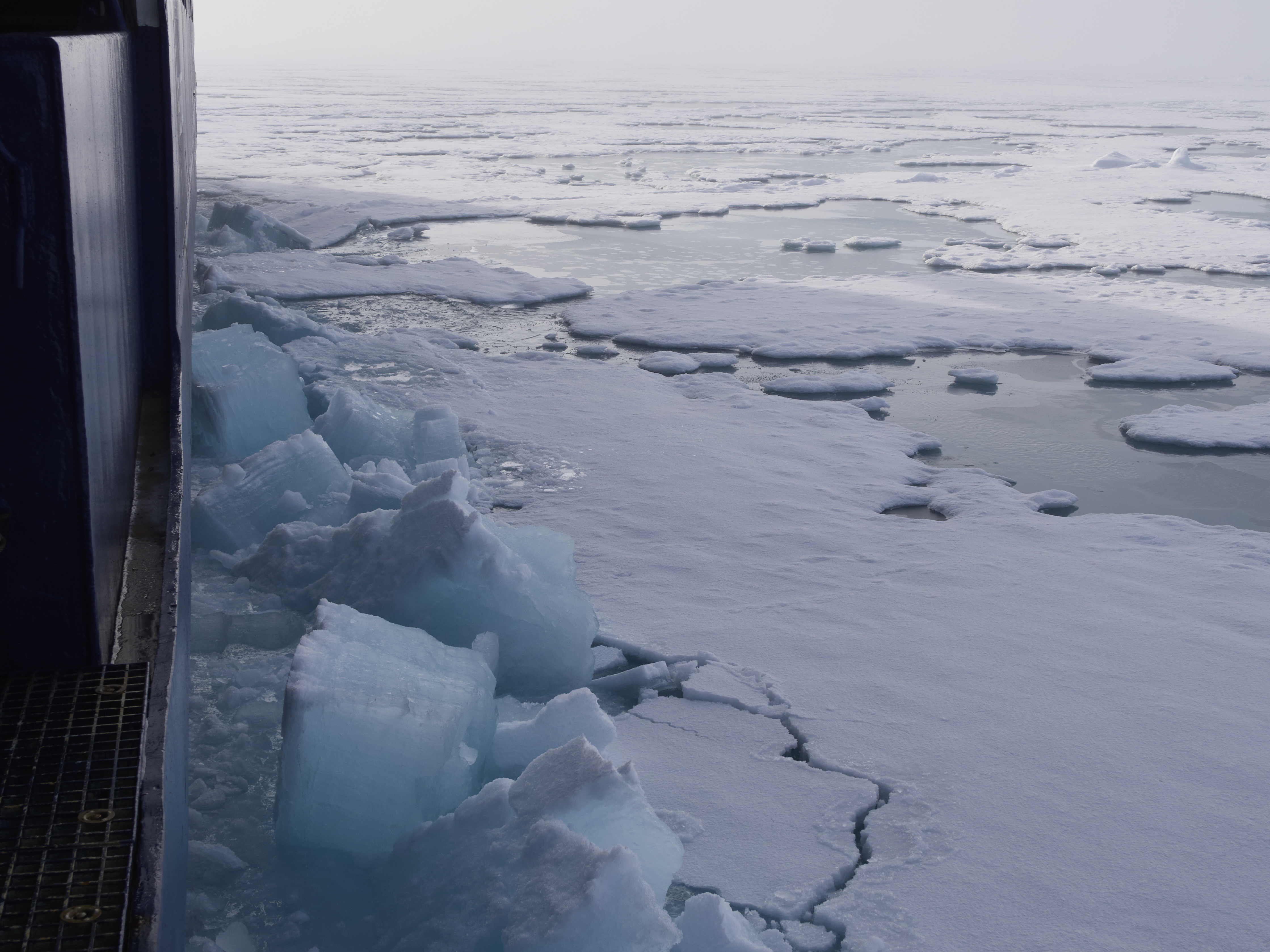
Although it was not necessary to break ice often between ice stations, it was still necessary at times. Thanks to daily satellite images and comparison with the ship's radar, ice-free zones were located very reliably and the transit time between stations was usually shorter than expected. (Photo: Matthias Jaggi / SLF)

Image 14 of 14
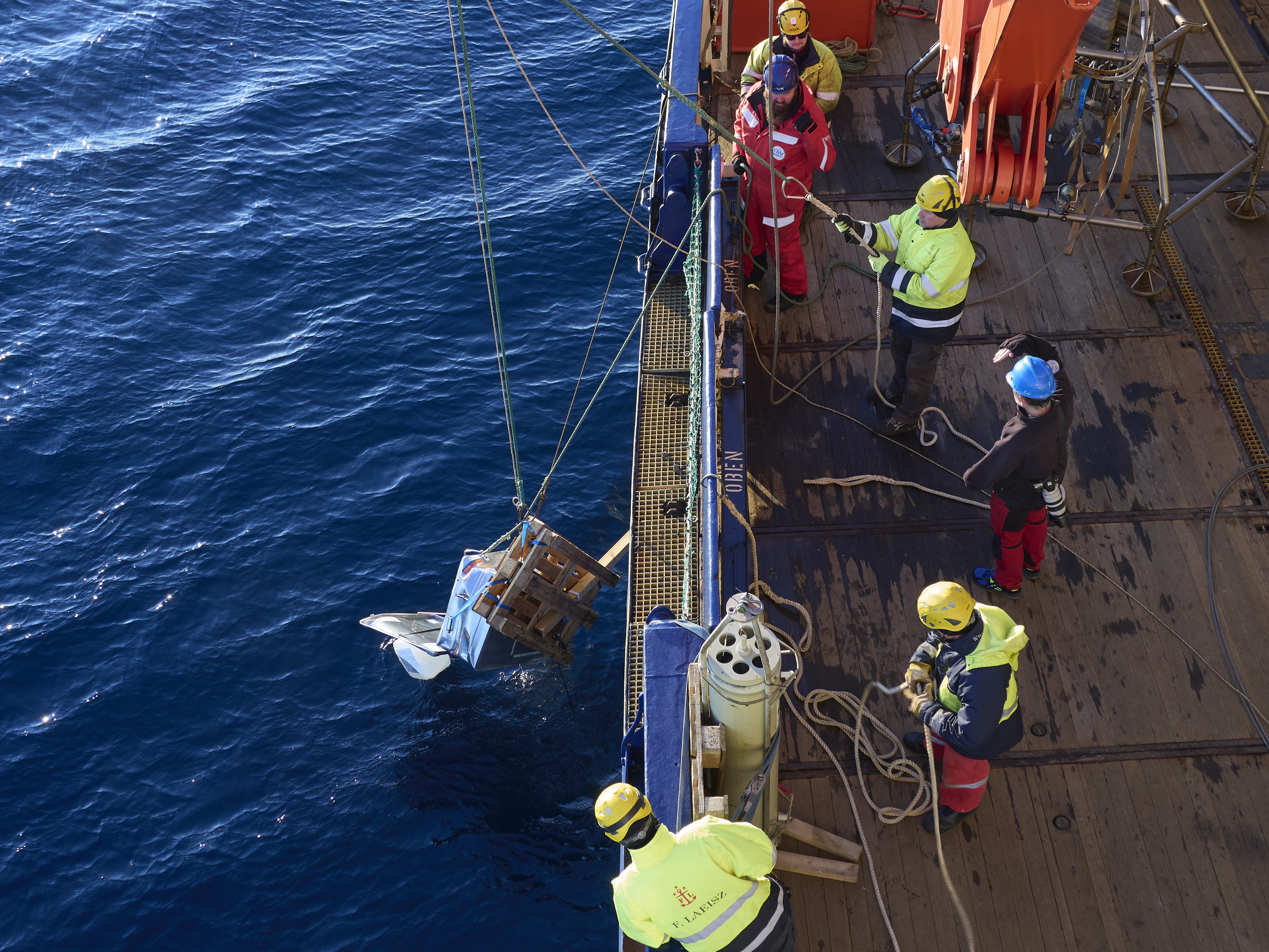
Rescue operation of autonomous measuring installations (buoys) from ice floe 1 in the peripheral zone, which broke apart completely after the third round. The buoys first drifted into Russian territory, where we were not allowed to go. Fortunately, however, they then drifted back into the Norwegian zone, where we were able to locate most of them and fish them out of the water. (Photo: Matthias Jaggi / SLF)
Links 
Copyright 
WSL and SLF provide image and sound material free of charge for use in press releases in connection with this media release. The use of this material in image, sound and/or video databases and the sale of the material by third parties is not permitted.